Type Type of Art in Cell A3 and Average of All Art in Cell A11

An array formula is a formula that can perform multiple calculations on one or more items in an assortment. You can think of an array every bit a row or column of values, or a combination of rows and columns of values. Assortment formulas can return either multiple results, or a single result.

Beginning with the September 2018 update for Microsoft 365, any formula that can return multiple results will automatically spill them either down, or across into neighboring cells. This change in behavior is besides accompanied past several new dynamic array functions. Dynamic array formulas, whether they're using existing functions or the dynamic array functions, merely demand to exist input into a single jail cell, then confirmed by pressing Enter. Earlier, legacy array formulas require first selecting the entire output range, and then confirming the formula with Ctrl+Shift+Enter. They're commonly referred to as CSE formulas.

You can use array formulas to perform circuitous tasks, such equally:

• Quickly create sample datasets.

• Count the number of characters contained in a range of cells.

• Sum only numbers that run into sure weather, such as the everyman values in a range, or numbers that fall between an upper and lower purlieus.

• Sum every Nth value in a range of values.

The following examples testify you how to create multi-prison cell and single-cell array formulas. Where possible, we've included examples with some of the dynamic array functions, as well as existing array formulas entered as both dynamic and legacy arrays.

Download our examples

Download an example workbook with all the array formula examples in this article.

This exercise shows you lot how to use multi-cell and unmarried-prison cell assortment formulas to summate a gear up of sales figures. The showtime set of steps uses a multi-cell formula to calculate a gear up of subtotals. The second set up uses a single-jail cell formula to calculate a grand total.

• Multi-jail cell array formula

  

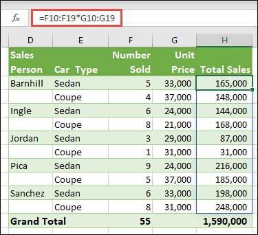
• Here nosotros're calculating Total Sales of coupes and sedans for each salesperson past entering =F10:F19*G10:G19 in jail cell H10.

  When you printing Enter, you'll run across the results spill down to cells H10:H19. Notice that the spill range is highlighted with a border when you select any cell within the spill range. You might also notice that the formulas in cells H10:H19 are grayed out. They're just in that location for reference, so if yous want to adjust the formula, you'll need to select cell H10, where the primary formula lives.

• Single-prison cell array formula

  

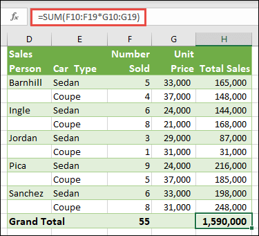
  In cell H20 of the example workbook, blazon or re-create and paste =SUM(F10:F19*G10:G19), and then press Enter.

  In this case, Excel multiplies the values in the array (the cell range F10 through G19), and then uses the SUM function to add the totals together. The event is a grand total of $1,590,000 in sales.

  This example shows how powerful this blazon of formula can be. For example, suppose you accept 1,000 rows of data. You tin can sum part or all of that data by creating an array formula in a single prison cell instead of dragging the formula down through the i,000 rows. Besides, find that the single-cell formula in jail cell H20 is completely independent of the multi-cell formula (the formula in cells H10 through H19). This is another advantage of using array formulas — flexibility. You could change the other formulas in column H without affecting the formula in H20. It can too be expert practice to have contained totals like this, as it helps validate the accuracy of your results.

• Dynamic assortment formulas also offer these advantages:

  • Consistency    If you click whatsoever of the cells from H10 downward, you encounter the same formula. That consistency can help ensure greater accuracy.

  • Safety    You can't overwrite a component of a multi-cell array formula. For example, click jail cell H11 and printing Delete. Excel won't modify the array's output. To change it, y'all demand to select the top-left prison cell in the array, or cell H10.

  • Smaller file sizes    Y'all can oft use a single array formula instead of several intermediate formulas. For instance, the car sales case uses one array formula to summate the results in column E. If you lot had used standard formulas such every bit =F10*G10, F11*G11, F12*G12, etc., you would have used 11 different formulas to summate the same results. That'due south not a big deal, but what if you had thousands of rows to total? Then information technology tin can make a large divergence.

  • Efficiency    Array functions can be an efficient way to build complex formulas. The array formula =SUM(F10:F19*G10:G19) is the same as this: =SUM(F10*G10,F11*G11,F12*G12,F13*G13,F14*G14,F15*G15,F16*G16,F17*G17,F18*G18,F19*G19).

  • Spilling    Dynamic array formulas will automatically spill into the output range. If your source information is in an Excel table, then your dynamic array formulas volition automatically resize as you add or remove information.

  • #SPILL! fault    Dynamic arrays introduced the #SPILL! mistake, which indicates that the intended spill range is blocked for some reason. When yous resolve the blockage, the formula will automatically spill.

Assortment constants are a component of assortment formulas. Yous create array constants by entering a list of items and and so manually surrounding the list with braces ({ }), similar this:

={i,two,3,4,5} or ={"Jan","February","March"}

If you split the items by using commas, you create a horizontal array (a row). If yous separate the items by using semicolons, you create a vertical array (a column). To create a two-dimensional array, you circumscribe the items in each row with commas, and delimit each row with semicolons.

The post-obit procedures will give you some practice in creating horizontal, vertical, and two-dimensional constants. We'll testify examples using the SEQUENCE part to automatically generate array constants, also as manually entered array constants.

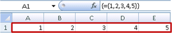
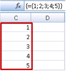
• Create a horizontal constant

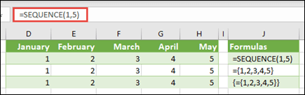
  Utilise the workbook from the previous examples, or create a new workbook. Select whatever empty cell and enter =SEQUENCE(one,5). The SEQUENCE function builds a 1 row by v column array the same as ={1,ii,3,four,5}. The following result is displayed:

  

• Create a vertical constant

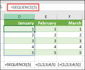
  Select any blank cell with room beneath information technology, and enter =SEQUENCE(5), or ={1;two;3;4;five}. The following result is displayed:

  

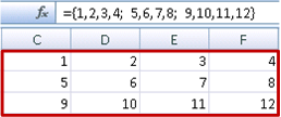
• Create a ii-dimensional constant

  Select any blank cell with room to the right and beneath it, and enter =SEQUENCE(3,iv). You see the post-obit outcome:

  

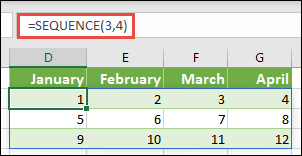
  You can also enter: or ={1,2,3,iv;v,6,7,8;ix,x,11,12}, merely you lot'll want to pay attending to where you put semi-colons versus commas.

  As you can encounter, the SEQUENCE choice offers pregnant advantages over manually entering your array constant values. Primarily, information technology saves y'all time, but information technology can too assist reduce errors from manual entry. It'southward as well easier to read, especially every bit the semi-colons can exist hard to distinguish from the comma separators.

Here's an example that uses array constants as office of a bigger formula. In the sample workbook, become to the Constant in a formula worksheet, or create a new worksheet.

In cell D9, we entered =SEQUENCE(one,5,3,1), merely you lot could besides enter three, four, 5, six, and seven in cells A9:H9. There's nothing special about that particular number selection, we just chose something other than 1-v for differentiation.

In cell E11, enter =SUM(D9:H9*SEQUENCE(1,5)), or =SUM(D9:H9*{1,2,3,4,5}). The formulas return 85.

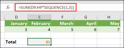
The SEQUENCE function builds the equivalent of the assortment constant {ane,2,3,4,v}. Because Excel performs operations on expressions enclosed in parentheses first, the side by side ii elements that come up into play are the cell values in D9:H9, and the multiplication operator (*). At this signal, the formula multiplies the values in the stored array by the corresponding values in the abiding. Information technology'due south the equivalent of:

=SUM(D9*ane,E9*2,F9*3,G9*4,H9*5), or =SUM(3*1,4*2,5*three,half-dozen*4,vii*5)

Finally, the SUM role adds the values, and returns 85.

To avoid using the stored array and keep the operation entirely in memory, you tin can replace information technology with another array constant:

=SUM(SEQUENCE(1,5,3,1)*SEQUENCE(1,5)), or =SUM({3,4,5,6,7}*{1,2,three,4,5})

Elements that y'all can employ in array constants

• Array constants can incorporate numbers, text, logical values (such as Truthful and Imitation), and error values such as #N/A. Y'all can use numbers in integer, decimal, and scientific formats. If you include text, you need to environment it with quotation marks ("text").

• Array constants tin can't contain additional arrays, formulas, or functions. In other words, they tin comprise only text or numbers that are separated by commas or semicolons. Excel displays a warning message when yous enter a formula such as {1,two,A1:D4} or {1,two,SUM(Q2:Z8)}. Also, numeric values can't incorporate per centum signs, dollar signs, commas, or parentheses.

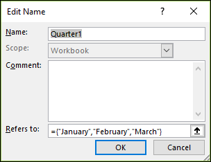
One of the best ways to utilise array constants is to name them. Named constants tin be much easier to employ, and they tin can hibernate some of the complication of your array formulas from others. To proper name an array constant and use it in a formula, do the following:

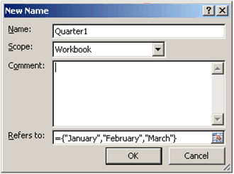
Go to Formulas > Defined Names > Define Name. In the Name box, blazon Quarter1. In the Refers to box, enter the following constant (recall to type the braces manually):

={"January","February","March"}

The dialog box should now wait like this:

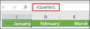
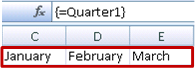
Click OK, then select whatever row with iii blank cells, and enter =Quarter1.

The following result is displayed:

If you desire the results to spill vertically instead of horizontally, yous can use =TRANSPOSE(Quarter1).

If y'all want to display a list of 12 months, like you might utilize when edifice a financial statement, you lot can base one off the electric current yr with the SEQUENCE office. The slap-up thing about this function is that fifty-fifty though merely the month is displaying, at that place is a valid date behind it that you lot can employ in other calculations. Yous'll find these examples on the Named array constant and Quick sample dataset worksheets in the case workbook.

=TEXT(DATE(YEAR(TODAY()),SEQUENCE(ane,12),1),"mmm")

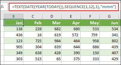
This uses the Appointment role to create a date based on the current year, SEQUENCE creates an array constant from one to 12 for January through December, then the TEXT function converts the display format to "mmm" (January, Feb, Mar, etc.). If you wanted to display the full calendar month name, such as January, you lot'd use "mmmm".

When yous apply a named abiding as an assortment formula, remember to enter the equal sign, equally in =Quarter1, not only Quarter1. If you don't, Excel interprets the array every bit a cord of text and your formula won't work as expected. Finally, keep in mind that you can apply combinations of functions, text and numbers. Information technology all depends on how creative you desire to get.

The following examples demonstrate a few of the means in which you can put assortment constants to apply in array formulas. Some of the examples use the TRANSPOSE function to catechumen rows to columns and vice versa.

• Multiple each item in an array

  Enter =SEQUENCE(1,12)*two, or ={one,2,3,4;five,half dozen,seven,8;9,ten,xi,12}*2

  You can also split with (/), add with (+), and decrease with (-).

• Square the items in an array

  Enter =SEQUENCE(1,12)^2, or ={1,ii,3,4;5,6,seven,8;9,10,eleven,12}^2

• Find the foursquare root of squared items in an array

  Enter =SQRT(SEQUENCE(1,12)^two), or =SQRT({ane,2,3,4;five,vi,7,8;9,10,11,12}^2)

• Transpose a one-dimensional row

  Enter =TRANSPOSE(SEQUENCE(1,v)), or =TRANSPOSE({i,2,3,4,five})

  Even though you entered a horizontal assortment constant, the TRANSPOSE office converts the array constant into a column.

• Transpose a one-dimensional column

  Enter =TRANSPOSE(SEQUENCE(v,1)), or =TRANSPOSE({1;2;3;4;5})

  Even though you entered a vertical array constant, the TRANSPOSE function converts the abiding into a row.

• Transpose a two-dimensional constant

  Enter =TRANSPOSE(SEQUENCE(iii,four)), or =TRANSPOSE({ane,ii,3,4;five,vi,vii,eight;nine,10,11,12})

  The TRANSPOSE function converts each row into a series of columns.

This section provides examples of basic assortment formulas.

• Create an array from existing values

  The following example explains how to use array formulas to create a new array from an existing array.

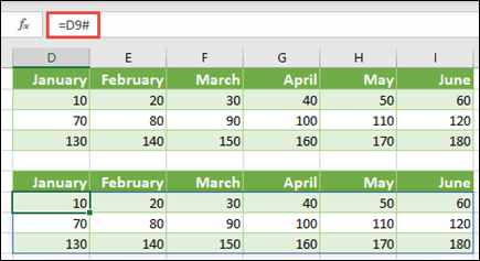
  Enter =SEQUENCE(3,6,10,10), or ={x,20,thirty,40,50,60;lxx,80,90,100,110,120;130,140,150,160,170,180}

  Be sure to blazon { (opening brace) before yous type 10, and } (closing caryatid) afterward y'all type 180, because you're creating an array of numbers.

  Next, enter =D9#, or =D9:I11 in a blank cell. A 3 x six array of cells appears with the aforementioned values you run across in D9:D11. The # sign is called the spilled range operator, and it's Excel's manner of referencing the unabridged array range instead of having to type information technology out.

  

• Create an array abiding from existing values

  Y'all can take the results of a spilled array formula and convert that into its component parts. Select cell D9, and then printing F2 to switch to edit manner. Next, printing F9 to convert the cell references to values, which Excel then converts into an array constant. When you press Enter, the formula, =D9#, should now be ={10,20,xxx;40,l,60;70,80,ninety}.

• Count characters in a range of cells

  The post-obit example shows y'all how to count the number of characters in a range of cells. This includes spaces.

  

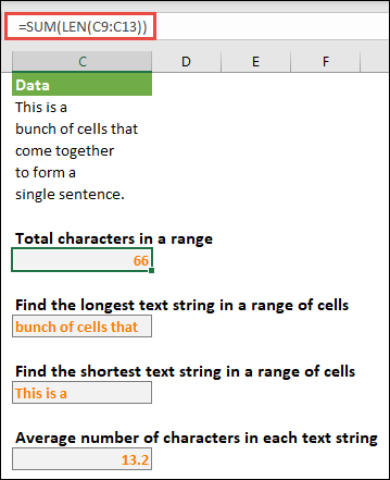
  =SUM(LEN(C9:C13))

  In this case, the LEN function returns the length of each text string in each of the cells in the range. The SUM function so adds those values together and displays the consequence (66). If yous wanted to get average number of characters, you could employ:

  =AVERAGE(LEN(C9:C13))

• Contents of longest prison cell in range C9:C13

  =INDEX(C9:C13,Lucifer(MAX(LEN(C9:C13)),LEN(C9:C13),0),i)

  This formula works only when a data range contains a single column of cells.

  Let's accept a closer look at the formula, starting from the inner elements and working outward. The LEN office returns the length of each of the items in the cell range D2:D6. The MAX part calculates the largest value amid those items, which corresponds to the longest text string, which is in cell D3.

  Here'southward where things get a little circuitous. The Match role calculates the offset (the relative position) of the jail cell that contains the longest text string. To practice that, it requires iii arguments: a lookup value, a lookup assortment, and a match blazon. The Lucifer office searches the lookup array for the specified lookup value. In this case, the lookup value is the longest text string:

  MAX(LEN(C9:C13)

  and that string resides in this assortment:

  LEN(C9:C13)

  The match blazon statement in this case is 0. The match type tin exist a i, 0, or -1 value.

  • 1 - returns the largest value that is less than or equal to the lookup val

  • 0 - returns the first value exactly equal to the lookup value

  • -1 - returns the smallest value that is greater than or equal to the specified lookup value

  • If you omit a match type, Excel assumes 1.

  Finally, the INDEX function takes these arguments: an assortment, and a row and column number within that array. The cell range C9:C13 provides the assortment, the Friction match office provides the cell address, and the final argument (ane) specifies that the value comes from the kickoff cavalcade in the assortment.

  If you wanted to get the contents of the smallest text string, you would replace MAX in the in a higher place example with MIN.

• Find the n smallest values in a range

  This example shows how to find the iii smallest values in a range of cells, where an assortment of sample data in cells B9:B18has been created with: =INT(RANDARRAY(10,one)*100). Note that RANDARRAY is a volatile function, then you'll get a new set of random numbers each fourth dimension Excel calculates.

  

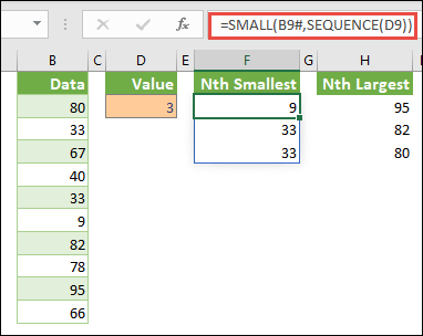
  Enter =Small(B9#,SEQUENCE(D9), =Minor(B9:B18,{one;two;iii})

  This formula uses an assortment constant to evaluate the Pocket-size part three times and return the smallest iii members in the assortment that's contained in cells B9:B18, where 3 is a variable value in cell D9. To find more than values, you tin can increment the value in the SEQUENCE function, or add more arguments to the constant. You can also utilise additional functions with this formula, such as SUM or AVERAGE. For case:

  =SUM(Pocket-size(B9#,SEQUENCE(D9))

  =Average(SMALL(B9#,SEQUENCE(D9))

• Detect the due north largest values in a range

  To find the largest values in a range, y'all can replace the SMALL function with the Large function. In add-on, the post-obit example uses the ROW and INDIRECT functions.

  Enter =Big(B9#,ROW(INDIRECT("1:3"))), or =Large(B9:B18,ROW(INDIRECT("1:three")))

  At this signal, it may help to know a bit about the ROW and INDIRECT functions. You tin can use the ROW function to create an array of consecutive integers. For example, select an empty and enter:

  =ROW(1:10)

  The formula creates a column of 10 consecutive integers. To see a potential problem, insert a row above the range that contains the array formula (that is, to a higher place row 1). Excel adjusts the row references, and the formula now generates integers from ii to xi. To ready that trouble, y'all add the INDIRECT role to the formula:

  =ROW(INDIRECT("ane:10"))

  The INDIRECT function uses text strings every bit its arguments (which is why the range 1:10 is surrounded by quotation marks). Excel does non suit text values when you insert rows or otherwise move the assortment formula. As a result, the ROW function always generates the array of integers that you want. Yous could merely as easily use SEQUENCE:

  =SEQUENCE(ten)

  Let'south examine the formula that you used earlier — =Large(B9#,ROW(INDIRECT("1:3"))) — starting from the inner parentheses and working outward: The INDIRECT part returns a set of text values, in this case the values 1 through 3. The ROW office in turn generates a three-cell column array. The LARGE function uses the values in the cell range B9:B18, and it is evaluated iii times, once for each reference returned by the ROW part. If y'all want to notice more than values, you add a greater prison cell range to the INDIRECT role. Finally, as with the Minor examples, you can use this formula with other functions, such as SUM and Average.

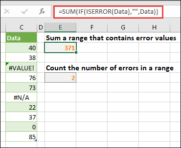
• Sum a range that contains fault values

  The SUM role in Excel does non work when you lot attempt to sum a range that contains an mistake value, such equally #VALUE! or #Northward/A. This example shows you how to sum the values in a range named Data that contains errors:

  

• =SUM(IF(ISERROR(Information),"",Information))

  The formula creates a new array that contains the original values minus whatever error values. Starting from the inner functions and working outward, the ISERROR function searches the jail cell range (Information) for errors. The IF role returns a specific value if a condition you specify evaluates to Truthful and some other value if it evaluates to FALSE. In this case, it returns empty strings ("") for all error values because they evaluate to Truthful, and it returns the remaining values from the range (Data) because they evaluate to FALSE, pregnant that they don't contain fault values. The SUM function then calculates the full for the filtered array.

• Count the number of mistake values in a range

  This example is like the previous formula, merely information technology returns the number of error values in a range named Data instead of filtering them out:

  =SUM(IF(ISERROR(Data),1,0))

  This formula creates an assortment that contains the value 1 for the cells that contain errors and the value 0 for the cells that don't contain errors. You can simplify the formula and achieve the aforementioned result past removing the tertiary statement for the IF function, like this:

  =SUM(IF(ISERROR(Information),1))

  If you don't specify the argument, the IF function returns Imitation if a prison cell does not contain an error value. You can simplify the formula even more than:

  =SUM(IF(ISERROR(Information)*1))

  This version works because TRUE*1=i and Simulated*1=0.

You might need to sum values based on atmospheric condition.

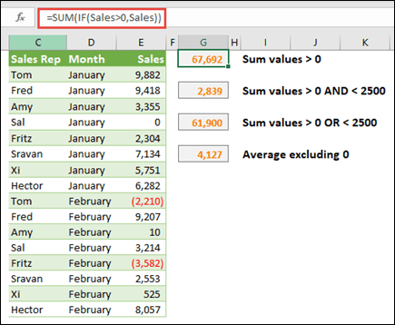
For example, this assortment formula sums simply the positive integers in a range named Sales, which represents cells E9:E24 in the example above:

=SUM(IF(Sales>0,Sales))

The IF part creates an array of positive and false values. The SUM part essentially ignores the false values considering 0+0=0. The prison cell range that you use in this formula can consist of whatsoever number of rows and columns.

You can also sum values that run across more than than one status. For example, this assortment formula calculates values greater than 0 AND less than 2500:

=SUM((Sales>0)*(Sales<2500)*(Sales))

Keep in heed that this formula returns an fault if the range contains one or more non-numeric cells.

You can likewise create assortment formulas that utilise a blazon of OR condition. For example, you lot tin can sum values that are greater than 0OR less than 2500:

=SUM(IF((Sales>0)+(Sales<2500),Sales))

You tin can't use the AND and OR functions in assortment formulas directly considering those functions return a single consequence, either Truthful or False, and array functions crave arrays of results. You can work effectually the problem by using the logic shown in the previous formula. In other words, you perform math operations, such as addition or multiplication on values that come across the OR or AND status.

This case shows you how to remove zeros from a range when you need to average the values in that range. The formula uses a data range named Sales:

=Boilerplate(IF(Sales<>0,Sales))

The IF office creates an array of values that practise non equal 0 and then passes those values to the Average function.

This array formula compares the values in two ranges of cells named MyData and YourData and returns the number of differences between the two. If the contents of the two ranges are identical, the formula returns 0. To apply this formula, the cell ranges need to exist the same size and of the same dimension. For example, if MyData is a range of iii rows by 5 columns, YourData must also be three rows past 5 columns:

=SUM(IF(MyData=YourData,0,1))

The formula creates a new array of the same size equally the ranges that you are comparison. The IF role fills the array with the value 0 and the value i (0 for mismatches and 1 for identical cells). The SUM function then returns the sum of the values in the array.

You can simplify the formula like this:

=SUM(1*(MyData<>YourData))

Like the formula that counts error values in a range, this formula works considering Truthful*1=one, and FALSE*1=0.

This array formula returns the row number of the maximum value in a single-cavalcade range named Data:

=MIN(IF(Data=MAX(Data),ROW(Data),""))

The IF function creates a new array that corresponds to the range named Information. If a corresponding cell contains the maximum value in the range, the assortment contains the row number. Otherwise, the array contains an empty string (""). The MIN role uses the new array as its 2nd argument and returns the smallest value, which corresponds to the row number of the maximum value in Data. If the range named Data contains identical maximum values, the formula returns the row of the commencement value.

If you want to render the bodily prison cell address of a maximum value, utilize this formula:

=Address(MIN(IF(Information=MAX(Data),ROW(Data),"")),COLUMN(Information))

You'll discover similar examples in the sample workbook on the Differences between datasets worksheet.

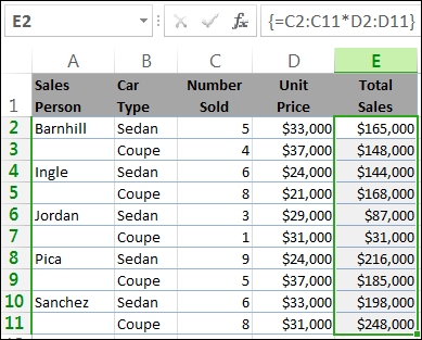
This practise shows you how to use multi-jail cell and single-cell assortment formulas to calculate a set of sales figures. The first ready of steps uses a multi-cell formula to summate a fix of subtotals. The second prepare uses a single-cell formula to calculate a grand total.

• Multi-cell array formula

Re-create the unabridged table beneath and paste it into cell A1 in a blank worksheet.

Sales Person	Car Blazon	Number Sold	Unit of measurement Price	Total Sales
Barnhill	Sedan	v	33000
	Coupe	iv	37000
Ingle	Sedan	vi	24000
	Coupe	eight	21000
Jordan	Sedan	3	29000
	Coupe	ane	31000
Pica	Sedan	9	24000
	Coupe	5	37000
Sanchez	Sedan	6	33000
	Coupe	8	31000
Formula (M Total)			K Total
'=SUM(C2:C11*D2:D11)			=SUM(C2:C11*D2:D11)

1. To see Total Sales of coupes and sedans for each salesperson, select cells E2:E11, enter the formula =C2:C11*D2:D11, and so press Ctrl+Shift+Enter.

2. To see the M Full of all sales, select cell F11, enter the formula =SUM(C2:C11*D2:D11), so press Ctrl+Shift+Enter.

When you press Ctrl+Shift+Enter, Excel surrounds the formula with braces ({ }) and inserts an instance of the formula in each jail cell of the selected range. This happens very quickly, then what you see in column Due east is the total sales amount for each car type for each salesperson. If you lot select E2, then select E3, E4, and then on, yous'll run into that the aforementioned formula is shown: {=C2:C11*D2:D11}.

• Create a unmarried-cell assortment formula

In prison cell D13 of the workbook, blazon the following formula, and then press Ctrl+Shift+Enter:

=SUM(C2:C11*D2:D11)

In this example, Excel multiplies the values in the array (the cell range C2 through D11) and then uses the SUM function to add the totals together. The result is a thou total of $i,590,000 in sales. This example shows how powerful this blazon of formula tin can exist. For example, suppose you lot have one,000 rows of information. You can sum part or all of that data by creating an array formula in a unmarried cell instead of dragging the formula down through the 1,000 rows.

Also, notice that the single-cell formula in cell D13 is completely independent of the multi-cell formula (the formula in cells E2 through E11). This is some other advantage of using array formulas — flexibility. Y'all could change the formulas in column E or delete that column altogether, without affecting the formula in D13.

Array formulas also offer these advantages:

• Consistency    If yous click any of the cells from E2 downward, you lot see the same formula. That consistency can assist ensure greater accuracy.

• Condom    You cannot overwrite a component of a multi-cell array formula. For example, click cell E3 and press Delete. You have to either select the entire range of cells (E2 through E11) and change the formula for the unabridged array, or get out the assortment as is. As an added condom mensurate, you have to printing Ctrl+Shift+Enter to confirm whatsoever change to the formula.

• Smaller file sizes    Yous can oft use a single array formula instead of several intermediate formulas. For case, the workbook uses one array formula to summate the results in column E. If you had used standard formulas (such every bit =C2*D2, C3*D3, C4*D4…), you lot would have used 11 unlike formulas to summate the same results.

In full general, array formulas use standard formula syntax. They all brainstorm with an equal (=) sign, and you tin can use most of the congenital-in Excel functions in your array formulas. The primal difference is that when using an array formula, you press Ctrl+Shift+Enter to enter your formula. When you lot exercise this, Excel surrounds your array formula with braces — if you type the braces manually, your formula will be converted to a text string, and it won't piece of work.

Array functions can be an efficient style to build circuitous formulas. The array formula =SUM(C2:C11*D2:D11) is the same equally this: =SUM(C2*D2,C3*D3,C4*D4,C5*D5,C6*D6,C7*D7,C8*D8,C9*D9,C10*D10,C11*D11).

Important:Press Ctrl+Shift+Enter whenever you demand to enter an array formula. This applies to both single-prison cell and multi-cell formulas.

Whenever you work with multi-jail cell formulas, also remember:

• Select the range of cells to hold your results before you enter the formula. You did this when you created the multi-jail cell assortment formula when yous selected cells E2 through E11.

• You can't change the contents of an individual cell in an array formula. To try this, select cell E3 in the workbook and press Delete. Excel displays a message that tells you lot that you can't alter role of an array.

• You tin move or delete an entire array formula, but you can't move or delete part of it. In other words, to shrink an assortment formula, yous first delete the existing formula and then beginning over.

• To delete an array formula, select the unabridged formula range (for example, E2:E11), then press Delete.

• Yous can't insert blank cells into, or delete cells from a multi-cell array formula.

At times, you may need to expand an array formula. Select the showtime jail cell in existing array range, and proceed until you've selected the entire range that you want to extend the formula to. Press F2 to edit the formula,  then press CTRL+SHIFT+ENTER to ostend the formula in one case yous've adapted the formula range. The key is to select the entire range, starting with the pinnacle-left cell in the array. The peak-left cell is the i that gets edited.

Array formulas are peachy, but they can take some disadvantages:

• You may occasionally forget to printing Ctrl+Shift+Enter. Information technology can happen to even the virtually experienced Excel users. Call up to press this key combination whenever you enter or edit an array formula.

• Other users of your workbook might not empathize your formulas. In exercise, assortment formulas are mostly not explained in a worksheet. Therefore, if other people need to change your workbooks, you lot should either avoid assortment formulas or make sure those people know about any array formulas and understand how to change them, if they demand to.

• Depending on the processing speed and retentivity of your calculator, large array formulas can slow downward calculations.

Array constants are a component of array formulas. You lot create assortment constants past entering a list of items and and so manually surrounding the list with braces ({ }), like this:

={i,2,three,4,5}

By now, yous know you lot need to printing Ctrl+Shift+Enter when you lot create array formulas. Because assortment constants are a component of array formulas, you environment the constants with braces by manually typing them. You then use Ctrl+Shift+Enter to enter the entire formula.

If y'all separate the items by using commas, you create a horizontal assortment (a row). If you split up the items by using semicolons, you create a vertical array (a column). To create a 2-dimensional array, y'all circumscribe the items in each row by using commas and circumscribe each row by using semicolons.

Here'due south an array in a single row: {i,ii,3,4}. Hither'south an array in a unmarried column: {1;ii;3;4}. And here's an array of two rows and four columns: {1,2,iii,4;v,6,7,viii}. In the ii row array, the first row is 1, two, 3, and 4, and the 2d row is 5, 6, 7, and 8. A single semicolon separates the two rows, betwixt four and five.

Every bit with array formulas, y'all tin can apply array constants with almost of the born functions that Excel provides. The following sections explain how to create each kind of constant and how to use these constants with functions in Excel.

The following procedures will give you lot some exercise in creating horizontal, vertical, and two-dimensional constants.

Create a horizontal constant

1. In a blank worksheet, select cells A1 through E1.

2. In the formula bar, enter the following formula, and then press Ctrl+Shift+Enter:

   ={1,2,three,4,5}

   In this case, you should type the opening and closing braces ({ }), and Excel will add together the second set for you.

   The post-obit outcome is displayed.

   

Create a vertical constant

1. In your workbook, select a cavalcade of five cells.

2. In the formula bar, enter the post-obit formula, and then press Ctrl+Shift+Enter:

   ={1;2;3;iv;5}

   The post-obit outcome is displayed.

   

Create a two-dimensional abiding

1. In your workbook, select a block of cells four columns wide by three rows high.

2. In the formula bar, enter the following formula, and then press Ctrl+Shift+Enter:

   ={1,2,3,4;5,6,7,8;9,ten,11,12}

   You lot run across the post-obit result:

   

Apply constants in formulas

Here is a unproblematic instance that uses constants:

1. In the sample workbook, create a new worksheet.

2. In cell A1, type 3, and and so blazon 4 in B1, 5 in C1, half-dozen in D1, and seven in E1.

3. In prison cell A3, type the post-obit formula, and then printing Ctrl+Shift+Enter:

   =SUM(A1:E1*{i,2,3,4,v})

   Notice that Excel surrounds the constant with another set of braces, because you entered information technology as an array formula.

   

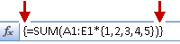
   The value 85 appears in prison cell A3.

The next section explains how the formula works.

The formula you lot merely used contains several parts.

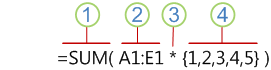
i. Function

two. Stored array

three. Operator

iv. Assortment abiding

The last element inside the parentheses is the assortment constant: {1,2,three,iv,5}. Remember that Excel does not surround array constants with braces; yous really type them. Also recall that after you add a constant to an array formula, you press Ctrl+Shift+Enter to enter the formula.

Because Excel performs operations on expressions enclosed in parentheses first, the next two elements that come into play are the values stored in the workbook (A1:E1) and the operator. At this bespeak, the formula multiplies the values in the stored array by the corresponding values in the constant. It's the equivalent of:

=SUM(A1*1,B1*two,C1*3,D1*4,E1*5)

Finally, the SUM function adds the values, and the sum 85 appears in cell A3.

To avoid using the stored array and to but keep the performance entirely in retentivity, replace the stored array with another array constant:

=SUM({3,four,5,six,7}*{1,ii,3,iv,five})

To try this, copy the part, select a blank cell in your workbook, paste the formula into the formula bar, and and so press Ctrl+Shift+Enter. Yous'll see the same result as you did in the earlier exercise that used the array formula:

=SUM(A1:E1*{1,ii,3,4,v})

Array constants can contain numbers, text, logical values (such equally TRUE and Imitation), and error values ( such equally #Northward/A). You tin use numbers in the integer, decimal, and scientific formats. If y'all include text, you need to surround the text with quotation marks (").

Assortment constants tin can't comprise additional arrays, formulas, or functions. In other words, they tin can contain only text or numbers that are separated by commas or semicolons. Excel displays a warning message when you enter a formula such as {1,2,A1:D4} or {i,2,SUM(Q2:Z8)}. Also, numeric values tin can't contain percent signs, dollar signs, commas, or parentheses.

I of the all-time way to utilise array constants is to name them. Named constants tin can be much easier to utilize, and they tin hibernate some of the complexity of your array formulas from others. To name an array constant and apply it in a formula, do the following:

1. On the Formulas tab, in the Defined Names group, click Define Proper noun.
   The Define Name dialog box appears.

2. In the Proper noun box, type Quarter1.

3. In the Refers to box, enter the following abiding (recollect to type the braces manually):

   ={"Jan","February","March"}

   The contents of the dialog box now looks like this:

   

4. Click OK, and so select a row of iii blank cells.

5. Type the following formula, and then press Ctrl+Shift+Enter.

   =Quarter1

   The following upshot is displayed.

   

When you apply a named constant as an assortment formula, remember to enter the equal sign. If you don't, Excel interprets the array as a string of text and your formula won't piece of work every bit expected. Finally, proceed in mind that you tin utilize combinations of text and numbers.

Look for the following problems when your array constants don't work:

• Some elements might not be separated with the proper grapheme. If y'all omit a comma or semicolon, or if you put one in the wrong place, the array constant might not be created correctly, or you might see a alert message.

• You might accept selected a range of cells that doesn't match the number of elements in your constant. For example, if you select a cavalcade of six cells for use with a v-cell constant, the #Northward/A error value appears in the empty cell. Conversely, if you select too few cells, Excel omits the values that don't have a corresponding prison cell.

The following examples demonstrate a few of the ways in which you tin put array constants to use in array formulas. Some of the examples use the TRANSPOSE function to convert rows to columns and vice versa.

Multiply each item in an assortment

1. Create a new worksheet, then select a block of empty cells four columns wide by 3 rows high.

2. Type the following formula, and then press Ctrl+Shift+Enter:

   ={one,2,3,four;5,6,7,8;9,10,11,12}*2

Square the items in an array

1. Select a block of empty cells four columns wide by three rows high.

2. Type the post-obit array formula, and so press Ctrl+Shift+Enter:

   ={1,ii,3,4;5,vi,7,8;ix,10,11,12}*{1,ii,3,four;5,6,vii,8;9,10,11,12}

   Alternatively, enter this array formula, which uses the caret operator (^):

   ={one,2,3,4;5,vi,vii,eight;9,10,11,12}^2

Transpose a one-dimensional row

1. Select a cavalcade of five bare cells.

2. Type the following formula, and and so printing Ctrl+Shift+Enter:

   =TRANSPOSE({ane,ii,3,4,5})

   Even though you entered a horizontal array constant, the TRANSPOSE function converts the array constant into a cavalcade.

Transpose a one-dimensional column

1. Select a row of five bare cells.

2. Enter the following formula, and so press Ctrl+Shift+Enter:

   =TRANSPOSE({ane;2;iii;4;5})

Even though y'all entered a vertical array constant, the TRANSPOSE function converts the constant into a row.

Transpose a two-dimensional constant

1. Select a cake of cells 3 columns wide by 4 rows high.

2. Enter the following abiding, and then press Ctrl+Shift+Enter:

   =TRANSPOSE({i,2,three,four;5,6,7,8;ix,x,11,12})

   The TRANSPOSE function converts each row into a series of columns.

This department provides examples of basic assortment formulas.

Create arrays and array constants from existing values

The following example explains how to utilize array formulas to create links between ranges of cells in different worksheets. It also shows you how to create an assortment abiding from the same ready of values.

Create an array from existing values

1. On a worksheet in Excel, select cells C8:E10, and enter this formula:

   ={10,twenty,xxx;twoscore,50,threescore;70,80,90}

   Be sure to type { (opening brace) before you type 10, and } (endmost brace) after you blazon 90, considering yous're creating an array of numbers.

2. Press Ctrl+Shift+Enter, which enters this array of numbers in the jail cell range C8:E10 by using an array formula. On your worksheet, C8 through E10 should look like this:

   10	twenty	30
   40	l	sixty
   70	fourscore	90

3. Select the jail cell range C1 through E3.

4. Enter the following formula in the formula bar, and then press Ctrl+Shift+Enter:

   =C8:E10

   A 3x3 array of cells appears in cells C1 through E3 with the aforementioned values you see in C8 through E10.

Create an array constant from existing values

1. With cells C1:C3 selected, printing F2 to switch to edit mode.

2. Press F9 to convert the cell references to values. Excel converts the values into an array constant. The formula should at present be ={x,20,30;40,50,60;70,80,90}.

3. Press Ctrl+Shift+Enter to enter the assortment abiding as an array formula.

Count characters in a range of cells

The following example shows you how to count the number of characters, including spaces, in a range of cells.

1. Re-create this entire tabular array and paste into a worksheet in cell A1.

   Data
   This is a
   bunch of cells that
   come up together
   to form a
   unmarried judgement.
   Total characters in A2:A6
   =SUM(LEN(A2:A6))
   Contents of longest prison cell (A3)
   =INDEX(A2:A6,MATCH(MAX(LEN(A2:A6)),LEN(A2:A6),0),1)

2. Select cell A8, and so press Ctrl+Shift+Enter to see the full number of characters in cells A2:A6 (66).

3. Select prison cell A10, then press Ctrl+Shift+Enter to see the contents of the longest of cells A2:A6 (cell A3).

The following formula is used in cell A8 counts the full number of characters (66) in cells A2 through A6.

=SUM(LEN(A2:A6))

In this instance, the LEN function returns the length of each text string in each of the cells in the range. The SUM role and then adds those values together and displays the effect (66).

Notice the northward smallest values in a range

This example shows how to find the three smallest values in a range of cells.

1. Enter some random numbers in cells A1:A11.

2. Select cells C1 through C3. This set of cells will hold the results returned past the array formula.

3. Enter the post-obit formula, and and so press Ctrl+Shift+Enter:

   =Modest(A1:A11,{ane;2;3})

This formula uses an array constant to evaluate the SMALL function iii times and render the smallest (1), 2nd smallest (2), and third smallest (3) members in the array that is contained in cells A1:A10 To find more values, y'all add more arguments to the constant. Yous tin also use boosted functions with this formula, such as SUM or Boilerplate. For instance:

=SUM(SMALL(A1:A10,{one,2,three})

=Average(SMALL(A1:A10,{1,2,3})

Detect the n largest values in a range

To find the largest values in a range, you can supercede the SMALL function with the LARGE function. In addition, the following example uses the ROW and INDIRECT functions.

1. Select cells D1 through D3.

2. In the formula bar, enter this formula, and so press Ctrl+Shift+Enter:

   =LARGE(A1:A10,ROW(INDIRECT("1:three")))

At this point, it may assistance to know a bit about the ROW and INDIRECT functions. You lot can use the ROW role to create an assortment of consecutive integers. For example, select an empty column of ten cells in your practice workbook, enter this array formula, and so press Ctrl+Shift+Enter:

=ROW(i:x)

The formula creates a column of 10 consecutive integers. To see a potential problem, insert a row higher up the range that contains the array formula (that is, higher up row 1). Excel adjusts the row references, and the formula generates integers from 2 to 11. To ready that problem, you add the INDIRECT role to the formula:

=ROW(INDIRECT("one:10"))

The INDIRECT function uses text strings as its arguments (which is why the range i:ten is surrounded past double quotation marks). Excel does non adjust text values when you insert rows or otherwise move the assortment formula. As a result, the ROW function e'er generates the array of integers that you want.

Let's accept a await at the formula that you used earlier — =Large(A5:A14,ROW(INDIRECT("1:iii"))) — starting from the inner parentheses and working outward: The INDIRECT function returns a set of text values, in this instance the values 1 through 3. The ROW office in plough generates a three-cell columnar array. The Large part uses the values in the cell range A5:A14, and it is evaluated three times, once for each reference returned by the ROW role. The values 3200, 2700, and 2000 are returned to the three-cell columnar array. If you want to notice more values, you add a greater cell range to the INDIRECT function.

As with earlier examples, y'all can apply this formula with other functions, such equally SUM and AVERAGE.

Find the longest text string in a range of cells

Go back to the before text string case, enter the post-obit formula in an empty cell, and press Ctrl+Shift+Enter:

=INDEX(A2:A6,Friction match(MAX(LEN(A2:A6)),LEN(A2:A6),0),ane)

The text "agglomeration of cells that" appears.

Permit'southward accept a closer look at the formula, starting from the inner elements and working outward. The LEN function returns the length of each of the items in the prison cell range A2:A6. The MAX role calculates the largest value among those items, which corresponds to the longest text string, which is in cell A3.

Here's where things get a niggling complex. The Match part calculates the offset (the relative position) of the cell that contains the longest text cord. To practice that, it requires three arguments: a lookup value, a lookup assortment, and a match type. The MATCH role searches the lookup array for the specified lookup value. In this case, the lookup value is the longest text string:

(MAX(LEN(A2:A6))

and that string resides in this array:

LEN(A2:A6)

The match type argument is 0. The match type can consist of a one, 0, or -one value. If you specify one, Match returns the largest value that is less than or equal to the lookup value. If y'all specify 0, Friction match returns the commencement value exactly equal to the lookup value. If you specify -1, Match finds the smallest value that is greater than or equal to the specified lookup value. If you omit a friction match type, Excel assumes 1.

Finally, the Index role takes these arguments: an array, and a row and cavalcade number inside that array. The jail cell range A2:A6 provides the array, the MATCH function provides the cell address, and the final argument (1) specifies that the value comes from the commencement column in the array.

This section provides examples of advanced assortment formulas.

Sum a range that contains fault values

The SUM function in Excel does not work when you try to sum a range that contains an fault value, such as #Due north/A. This example shows you how to sum the values in a range named Data that contains errors.

=SUM(IF(ISERROR(Information),"",Data))

The formula creates a new array that contains the original values minus any mistake values. Starting from the inner functions and working outward, the ISERROR function searches the cell range (Information) for errors. The IF part returns a specific value if a condition you specify evaluates to Truthful and another value if it evaluates to Simulated. In this case, it returns empty strings ("") for all mistake values because they evaluate to Truthful, and information technology returns the remaining values from the range (Data) because they evaluate to Faux, pregnant that they don't incorporate mistake values. The SUM function then calculates the total for the filtered array.

Count the number of fault values in a range

This example is like to the previous formula, but it returns the number of fault values in a range named Data instead of filtering them out:

=SUM(IF(ISERROR(Information),i,0))

This formula creates an assortment that contains the value 1 for the cells that incorporate errors and the value 0 for the cells that don't contain errors. You can simplify the formula and achieve the same issue past removing the third argument for the IF function, like this:

=SUM(IF(ISERROR(Data),1))

If you lot don't specify the statement, the IF function returns Simulated if a jail cell does not contain an error value. You can simplify the formula fifty-fifty more:

=SUM(IF(ISERROR(Information)*1))

This version works because TRUE*i=1 and False*one=0.

Sum values based on weather condition

You might need to sum values based on atmospheric condition. For example, this assortment formula sums just the positive integers in a range named Sales:

=SUM(IF(Sales>0,Sales))

The IF function creates an array of positive values and false values. The SUM role substantially ignores the false values because 0+0=0. The cell range that you use in this formula tin consist of whatever number of rows and columns.

You can also sum values that run across more than 1 condition. For example, this array formula calculates values greater than 0 and less than or equal to 5:

=SUM((Sales>0)*(Sales<=5)*(Sales))

Keep in listen that this formula returns an error if the range contains one or more non-numeric cells.

You can also create array formulas that use a blazon of OR condition. For example, you tin sum values that are less than 5 and greater than 15:

=SUM(IF((Sales<5)+(Sales>fifteen),Sales))

The IF function finds all values smaller than five and greater than 15 and then passes those values to the SUM part.

Yous can't use the AND and OR functions in assortment formulas directly considering those functions return a single result, either TRUE or FALSE, and array functions crave arrays of results. Yous can work around the problem past using the logic shown in the previous formula. In other words, you perform math operations, such every bit improver or multiplication, on values that run across the OR or AND condition.

Compute an average that excludes zeros

This example shows you how to remove zeros from a range when y'all need to average the values in that range. The formula uses a data range named Sales:

=AVERAGE(IF(Sales<>0,Sales))

The IF function creates an array of values that do not equal 0 and so passes those values to the AVERAGE function.

Count the number of differences betwixt two ranges of cells

This array formula compares the values in two ranges of cells named MyData and YourData and returns the number of differences betwixt the 2. If the contents of the two ranges are identical, the formula returns 0. To apply this formula, the cell ranges need to exist the aforementioned size and of the same dimension (for example, if MyData is a range of three rows by v columns, YourData must likewise be 3 rows by v columns):

=SUM(IF(MyData=YourData,0,one))

The formula creates a new array of the same size equally the ranges that you lot are comparing. The IF function fills the array with the value 0 and the value 1 (0 for mismatches and 1 for identical cells). The SUM function so returns the sum of the values in the array.

You can simplify the formula like this:

=SUM(1*(MyData<>YourData))

Similar the formula that counts error values in a range, this formula works because TRUE*i=1, and FALSE*1=0.

Find the location of the maximum value in a range

This array formula returns the row number of the maximum value in a single-column range named Data:

=MIN(IF(Data=MAX(Information),ROW(Information),""))

The IF function creates a new array that corresponds to the range named Information. If a corresponding cell contains the maximum value in the range, the array contains the row number. Otherwise, the array contains an empty string (""). The MIN office uses the new assortment as its second argument and returns the smallest value, which corresponds to the row number of the maximum value in Data. If the range named Data contains identical maximum values, the formula returns the row of the first value.

If you lot want to return the actual cell accost of a maximum value, use this formula:

=ADDRESS(MIN(IF(Data=MAX(Data),ROW(Data),"")),COLUMN(Data))

Acknowledgement

Parts of this article were based on a series of Excel Power User columns written past Colin Wilcox, and adapted from chapters 14 and xv of Excel 2002 Formulas, a book written by John Walkenbach, a former Excel MVP.

Demand more than assistance?

You can always ask an practiced in the Excel Tech Community or get support in the Answers customs.

See Also

Dynamic arrays and spilled array behavior

Dynamic array formulas vs. legacy CSE array formulas

FILTER office

RANDARRAY function

SEQUENCE office

SORT office

SORTBY function

UNIQUE function

#SPILL! errors in Excel

Implicit intersection operator: @

Overview of formulas

eastwrible.blogspot.com

Source: https://support.microsoft.com/en-us/office/guidelines-and-examples-of-array-formulas-7d94a64e-3ff3-4686-9372-ecfd5caa57c7

Share this post